Jupyter Snippet CB2nd 04_sde

13.4. Simulating a stochastic differential equation

import numpy as np
import matplotlib.pyplot as plt
%matplotlib inline

sigma = 1.  # Standard deviation.
mu = 10.  # Mean.
tau = .05  # Time constant.

dt = .001  # Time step.
T = 1.  # Total time.
n = int(T / dt)  # Number of time steps.
t = np.linspace(0., T, n)  # Vector of times.

sigma_bis = sigma * np.sqrt(2. / tau)
sqrtdt = np.sqrt(dt)

x = np.zeros(n)

for i in range(n - 1):
    x[i + 1] = x[i] + dt * (-(x[i] - mu) / tau) + \
        sigma_bis * sqrtdt * np.random.randn()

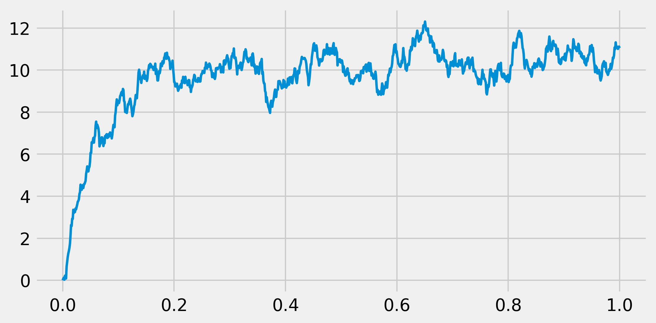
fig, ax = plt.subplots(1, 1, figsize=(8, 4))
ax.plot(t, x, lw=2)

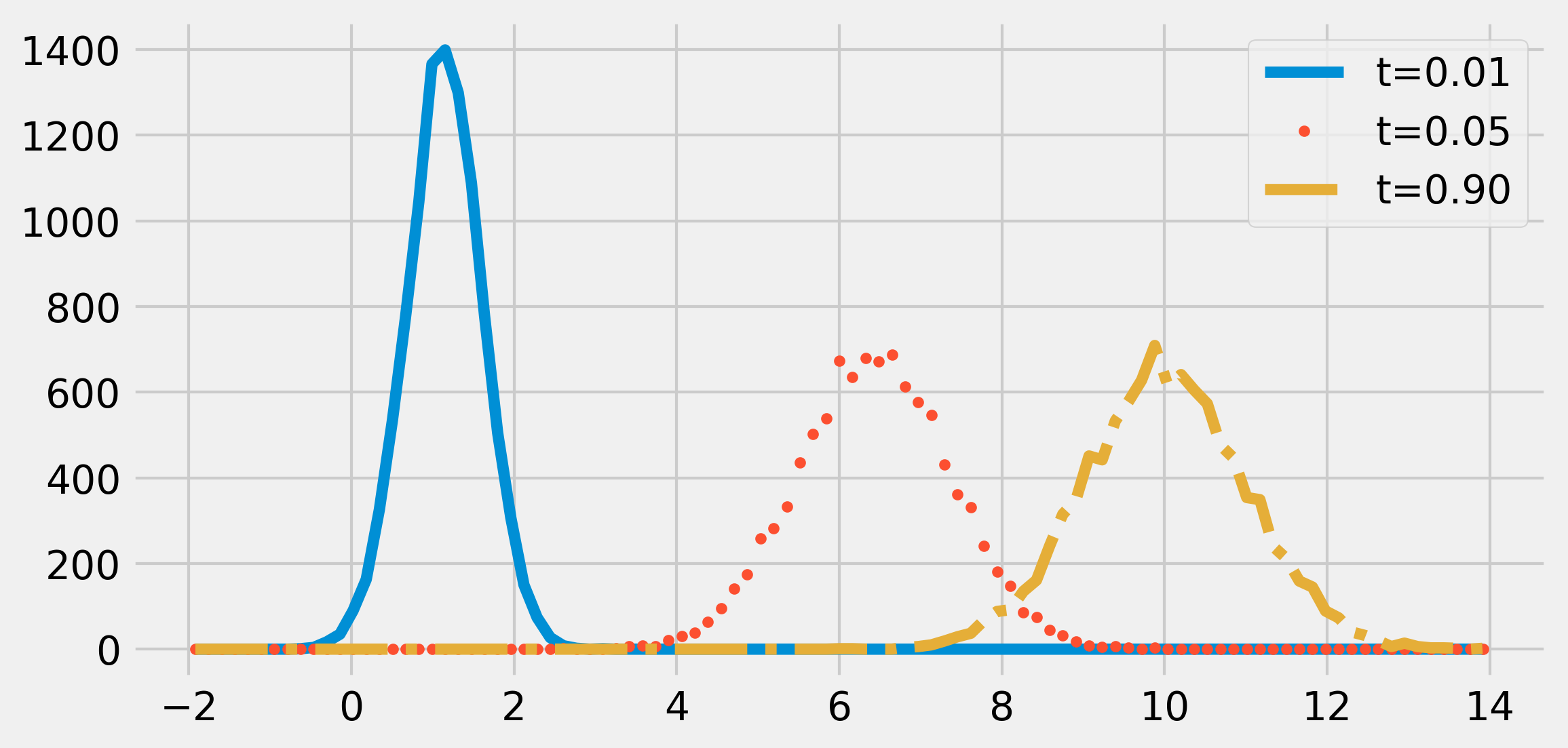
ntrials = 10000
X = np.zeros(ntrials)

# We create bins for the histograms.
bins = np.linspace(-2., 14., 100)
fig, ax = plt.subplots(1, 1, figsize=(8, 4))
for i in range(n):
    # We update the process independently for
    # all trials
    X += dt * (-(X - mu) / tau) + \
        sigma_bis * sqrtdt * np.random.randn(ntrials)
    # We display the histogram for a few points in
    # time
    if i in (5, 50, 900):
        hist, _ = np.histogram(X, bins=bins)
        ax.plot((bins[1:] + bins[:-1]) / 2, hist,
                {5: '-', 50: '.', 900: '-.', }[i],
                label=f"t={i * dt:.2f}")
    ax.legend()